PANEL METHOD of HESS and SMITH

Vortex Flow

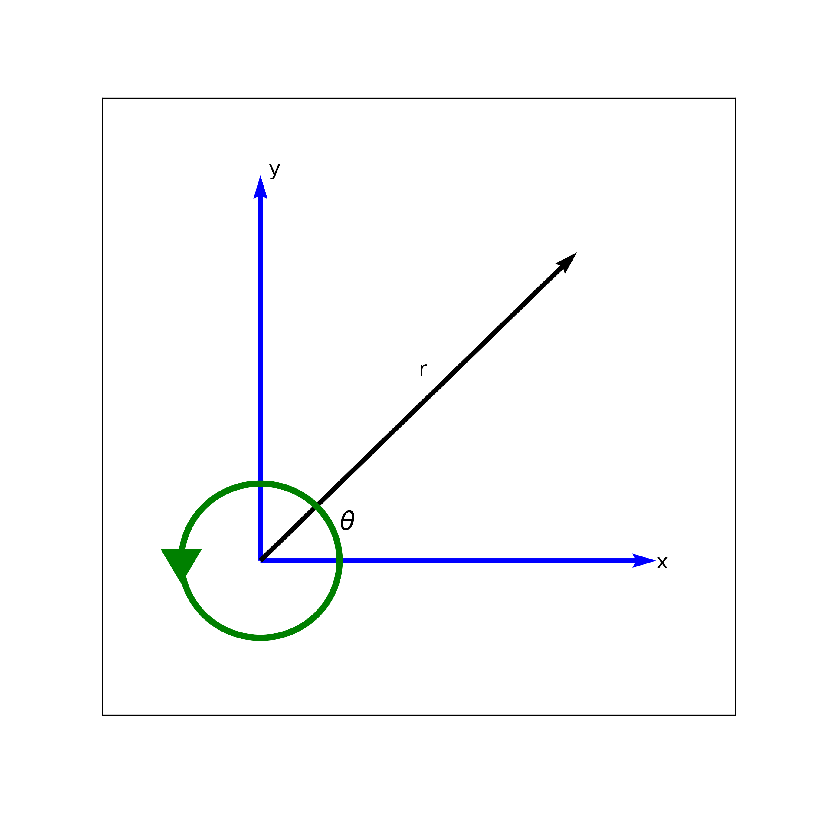
Let a point vortex be places at the origin Then the velocity components will be $$v_{r} = 0$$

$$v_{\theta}=\frac{C}{r}$$

In contrast to source flow, for the vortex flow the, the flow field is incompressible everywhere and irrotatinonal everywhere except at the origin. From the definition of circulation we can find the constant C in the tangential velocity component

$$\Gamma=-\oint \textbf{V}\cdot d\textbf{S}=-\oint v_{\theta}rd\theta=-v_{\theta}2\pi r$$$$v_{\theta}=\frac{-\Gamma}{2\pi r}$$

In here, $\Gamma$ is the strength of the vortex flow. Using the Stoke's theroem we can find the circulation in terms of vorticity

$$\Gamma=-\oint_{C}\textbf{V}\cdot d\textbf{S}=-\int \int (\nabla \times \textbf{V})\cdot d\textbf{S}$$

The potential induced by the vorticity can be calculated from the velocity components

$$u_{r}=\frac{\partial \phi}{\partial r}=0 \rightarrow \phi = c_{1}+f(\theta)$$

$$u_{\theta}=\frac{1}{r}\frac{\partial \phi}{\partial \theta}=\frac{-\Gamma}{2\pi r} \rightarrow \phi = \frac {-\Gamma}{2\pi}\theta = f(r)$$
Then the velocity potential due to vorticity reads $$\phi_{v} = \frac{-\Gamma}{2\pi}\theta $$

Vortex Sheet

Let $\gamma=\gamma(s)$ be the vortex shhet strength per unit length.

$$\Gamma=\int_{a}^{b}\gamma ds$$

$\gamma ds$ induces a velocity at point P such that

$$dv=\frac{-\gamma ds}{2\pi r} \rightarrow d\phi=\frac{-\gamma ds}{2\pi}\theta$$

Then the total velocity potential is

$$\phi(x,y) = \int_{a}^{b}\frac{-\gamma dS}{2\pi}\theta = -\frac{1}{2\pi}\int_{a}^{b}\gamma \theta dS$$

Now, calculate the circulation for this vortex sheet

$$\Gamma=-\oint \textbf{V}\cdot d\textbf{S}=\left[ (v_{2}dn)-(u_{1}ds)-(v_{1}dn)+(u_{2}ds)\right]=(u_{1}-u_{2})ds+(v_{1}-v_{2})dn=\int \gamma ds$$

Therefore $$\gamma ds=(u_{1}-u_{2})ds+(v_{1}-v_{2})dn$$

In order to represent the actual vortex sheet, we let $dn\rightarrow 0$

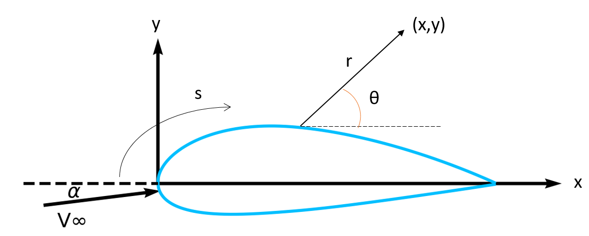
$$\gamma ds = (u_{1}-u_{2})ds \rightarrow \gamma = u_{1}-u_{2}$$

The surface of the airfoil is represented by source and vortex distributions. The total potential around the airfoil is the sum of the potentials due to free stream, source distribution and vortex distribution. $$\phi=\phi_{\infty}+\phi_{s}+\phi_{v}$$

$$\phi=V_{\infty}[xcos\alpha+ysin\alpha]+\int\frac{q(s)}{2\pi}\ln r ds-\int \frac{\gamma(s)}{2\pi}\theta ds$$

where the source and vortex distributions are integrated over the airfoil surface. Since each of these potentials satisfy $\nabla^{2}\phi=0$ and the far field boundary conditions, the total potential also satisfies. The unique solution is determined after applying the flow tangency and the Kutta condition.

$$\textrm{q(s)} \rightarrow \textrm{from flow tangency}$$

$$\gamma(s) \rightarrow \textrm{from Kutta condition}$$

By the representation of the airfoil surface with panels as shown in the figure below, the potential becomes as follows:

$$\phi=V_{\infty}[xcos\alpha+ysin\alpha]+\sum_{j=1}^{N}\int_{j}\frac{q(s)}{2\pi}\ln r ds-\sum_{j=1}^{N}\int_{j} \frac{\gamma}{2\pi}\theta ds$$

The unique solution is only obtained by a specific value of circulation, therefore vortex strength distribution $\gamma(s)$ is replaced by the specific value $\gamma$ which satisfies the Kutta condition.



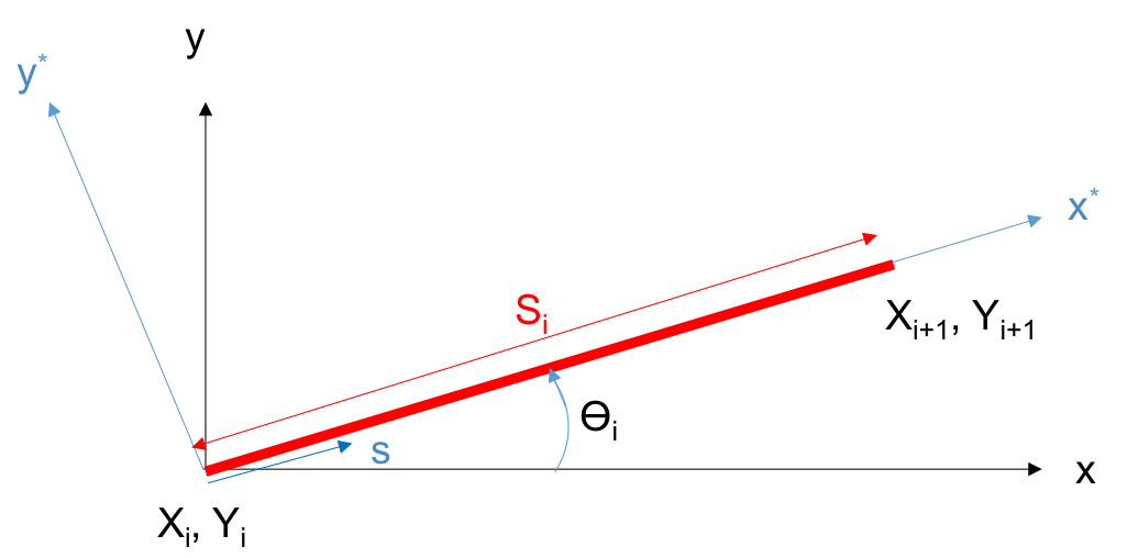
Using the geometric properties of the panel shown in the figure, we can find the angle $\theta _{i}$, the normal vector $\textbf{n}_{j}$ and the tangent vector $\textbf{t}_{j}$ as follows

$$\sin \theta_{i}=\frac{Y_{i+1}-Y_{i}}{S_{i}}\hspace{5pt},\hspace{5pt}\cos \theta_{i}=\frac{X_{i+1}-X_{i}}{S_{i}}$$

$$\textbf{n}_{i}=-\sin \theta_{i}\hat{i}+\cos \theta_{i}\hat{j}$$

$$\textbf{t}_{i}=\cos \theta_{i}\hat{i}+\sin \theta_{i}\hat{j}$$

Let $u_{i}$ and $v_{i}$ be the $x$ and $y$ component of the velocity at the mid point of the panel. The flow tangency condition is $\textbf{V}\cdot\textbf{n}=0$

$$\left\{\begin{array}{c} u_{i}\\ v_{i} \end{array} \right\}\cdot\left\{\begin{array}{c} -\sin \theta_{i}\\ \cos \theta_{i} \end{array} \right\}=-u_{i}\sin \theta_{i}+v_{i}\cos \theta_{i}=0$$

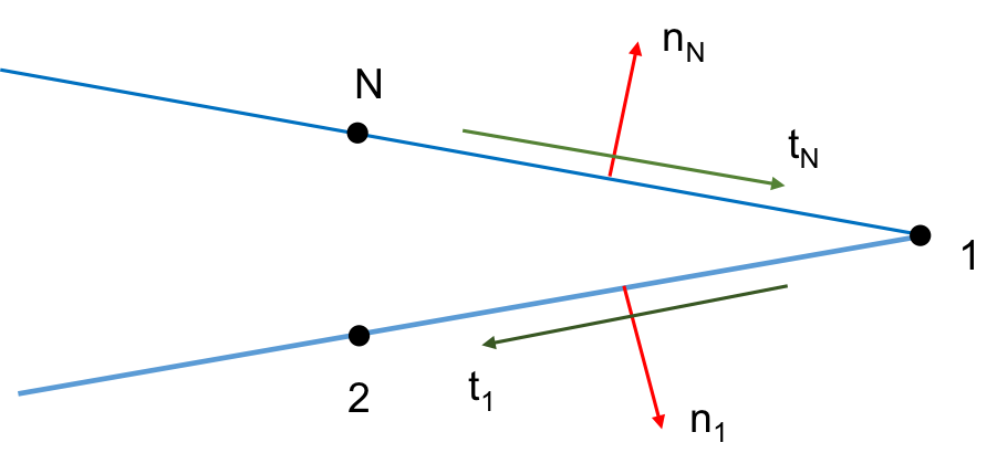
And the Kutta condition becomes $[\textbf{V}\cdot \textbf{t}]_{1}=[\textbf{V}\cdot\textbf{t}]_{2}$

$$\left\{\begin{array}{c} u_{1}\\ v_{1} \end{array} \right\}\cdot\left\{\begin{array}{c} \cos \theta_{1}\\ \sin \theta_{1} \end{array} \right\}=\left\{\begin{array}{c} u_{N}\\ v_{N} \end{array} \right\}\cdot\left\{\begin{array}{c} \cos \theta_{N}\\ \sin \theta_{N} \end{array} \right\}$$

$$u_{1}\cos \theta_{1}+v_{1}\sin \theta_{1}=-u_{N}\cos \theta_{N}-v_{N}\sin \theta_{N}$$



The velocity components at any given point are calculated as follows

$$u_{i}=V_{\infty}\cos \alpha+\sum_{j=1}^{N}q_{j}IU_{ij}+\sum_{j=1}^{N}\gamma JU_{ij}$$

$$v_{i}=V_{\infty}\sin \alpha+\sum_{j=1}^{N}q_{j}IV_{ij}+\sum_{j=1}^{N}\gamma JV_{ij}$$

In here, $IU_{ij}$ and $IV_{ij}$ are velocity coefficients induced by source distribution and $JU_{ij}$ and $JV_{ij}$ are the velocity coefficients induced by the vortex strength due to panel $j$ . And the velocity components can be written in terms of local coordinate system velocities $u^{*}$ and $v^{*}$ of panel $j$.

$$u=u^{*}\cos\theta_{j}-v^{*}\sin\theta_{j}$$

$$v=u^{*}\sin\theta_{j}+u^{*}\cos\theta_{j}$$

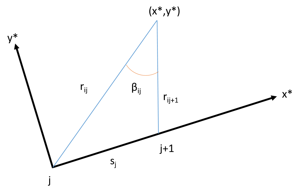
The placement of the source distribution $q(s)$ at any point $s$ along the $x^{*}$ axis gives $IU$ and $IV$ as follows

$$IU_{ij} = \frac{1}{2\pi}\int_{0}^{S_{j}}\frac{x_{i}^{*}-s}{(x_{i}^{*}-s)^{2}+y_{i}^{2}}ds=-\frac{1}{2\pi}\left.\ln\left[(x_{i}^{*}-s)^{2}+(y_{i}^{*})^{2}\right]^{0.5}\right|_{0}^{S_{j}}=-\frac{1}{2\pi}\ln\left[\frac{r_{i,j+1}}{r_{ij}}\right]$$

$$IV_{ij} = \frac{1}{2\pi}\int_{0}^{S_{j}}\frac{y_{i}^{*}}{(x_{i}^{*}-s)^{2}+y_{i}^{2}}ds=\frac{1}{2\pi}\left.\arctan\left[\frac{y_{i}^{*}}{x_{i}^{*}-s}\right]\right|_{0}^{S_{j}}=\frac{\beta_{ij}}{2\pi}$$

As can be seen in the figure $r_{ij }$ is the distance between $(X_{j},Y_{j})$ and $(x_{i},y_{i})$ and $r_{i,j+1 }$ is the distance between $(X_{j+1},Y_{j+1})$ and $(x_{i},y_{i})$. As point $i$ and $j$ coincide, $r_{ij }$ and $r_{i,j+1 }$ become equal and $IU_{ii}$ goes to zero. And the angle $\beta_{ii}$ goes to $\pi$ and $IV_{ii}=1/2$. Similarly the induced velocities due to $\gamma$ at point $(x_{i}^{*},y_{i}^{*})$ can be written as follows

$$JU_{ij} = -\frac{1}{2\pi}\int_{0}^{S_{i}}\frac{y_{i}^{*}}{(x_{i}^{*}-s)^{2}+y_{i}^{2}}ds=\frac{\beta_{ij}}{2\pi}$$

$$JV_{ij} = -\frac{1}{2\pi}\int_{0}^{S_{i}}\frac{(x_{i}^{*}-s)}{(x_{i}^{*}-s)^{2}+y_{i}^{2}}ds=\frac{1}{2\pi}\ln\left[\frac{r_{i,j+1}}{r_{ij}}\right]$$



All these equations construct the linear system as follows

$$\sum_{j=1}^{N}A_{ij}q_{j}+A_{1,N+1}\gamma=b_{i}$$

$$\sum_{j=1}^{N}A_{N+1,j}q_{j}+A_{N+1,N+1}\gamma=b_{N+1}$$

The coefficient matrices and the RHS vector are as follows

$$A_{ij}=\frac{1}{2\pi}\left[\sin(\theta_{i}-\theta_{j})\ln\frac{r_{i,j+1}}{r_{ij}}+\cos(\theta_{i}-\theta_{j})\beta_{ij}\right]$$

$$A_{i,N+1}=\frac{1}{2\pi}\sum_{j=1}^{N}\left[cos(\theta_{i}-\theta_{j})\ln\frac{r_{i,j+1}}{r_{ij}}-\sin(\theta_{i}-\theta_{j})\beta_{ij}\right]$$

$$A_{N+1,j}=\frac{1}{2\pi}\sum_{k=1,N}\left[sin(\theta_{k}-\theta_{j})\beta_{kj}-\cos(\theta_{k}-\theta_{j})\ln\frac{r_{k,j+1}}{r_{kj}}\right]$$

$$A_{N+1,N+1}=\frac{1}{2\pi}\sum_{k=1,N}\sum_{j=1}^{N}\left[sin(\theta_{k}-\theta_{j})\ln\frac{r_{k,j+1}}{r_{kj}}+\cos(\theta_{k}-\theta_{j})\beta_{kj}\right]$$

$$b_{i}=V_{\infty}\sin(\theta_{i}-\alpha)$$

$$b_{N+1}=-V_{\infty}\left[\cos(\theta_{1}-\alpha)+\cos(\theta_{N}-\alpha)\right]$$

The matrix form of the linear system is

$$\left[\begin{array}{ccccccc|c} & & & & & & & \\ & & & & & & & \\ & & & & & & & \\ & & A_{ij}& & & & & A_{i,N+1} \\ & & & & & & & \\ & & & & & & & \\ & & & & & & & \\ \hline & &A_{N+1,j} & & & & & A_{N+1,N+1} \end{array}\right]\left\{\begin{array}{c} q_{1}\\ q_{2}\\ \\ \vdots\\ \\ q_{N-1}\\ q_{N}\\ \hline \gamma \end{array} \right\}=\left\{\begin{array}{c} b_{1}\\ b_{2}\\ \\ \vdots\\ \\ b_{N-1}\\ b_{N}\\ \hline b_{N+1} \end{array} \right\}$$

Once the system is solved, the tangential velocities are computed from the following equations

$$ V_{ti}=\textbf{V}\cdot\textbf{t}=V_{\infty}\cos(\theta_{i}-\alpha)+\sum_{j=1}^{N}\frac{q_{j}}{2\pi}\left[sin(\theta_{i}-\theta_{j})\beta_{ij}-\cos(\theta_{i}-\theta_{j})\ln\frac{r_{i,j+1}}{r_{ij}}\right]\\ +\frac{\gamma}{2\pi}\sum_{j=1}^{N}\left[sin(\theta_{i}-\theta_{j})\ln\frac{r_{i,j+1}}{r_{ij}}+\cos(\theta_{i}-\theta_{j})\beta_{ij}\right]$$

<< 4.1.1 Example: Non-Lifting Flow Over a Circular Cylinder || Contents || 4.2.1 Example: Lifting Flow Over Airfoils >>

References:

[1] An Introduction to Theoretical and Computational Aerodynamics, Jack Moran, Dover Publications, 2010.

[2] Theoretical and Experimental Aerodynamics, Mrinal Kaushik, Springer, 2019.

Created using Jupyter Notebook