Non-Lifting Flow Over a Circular Cylinder
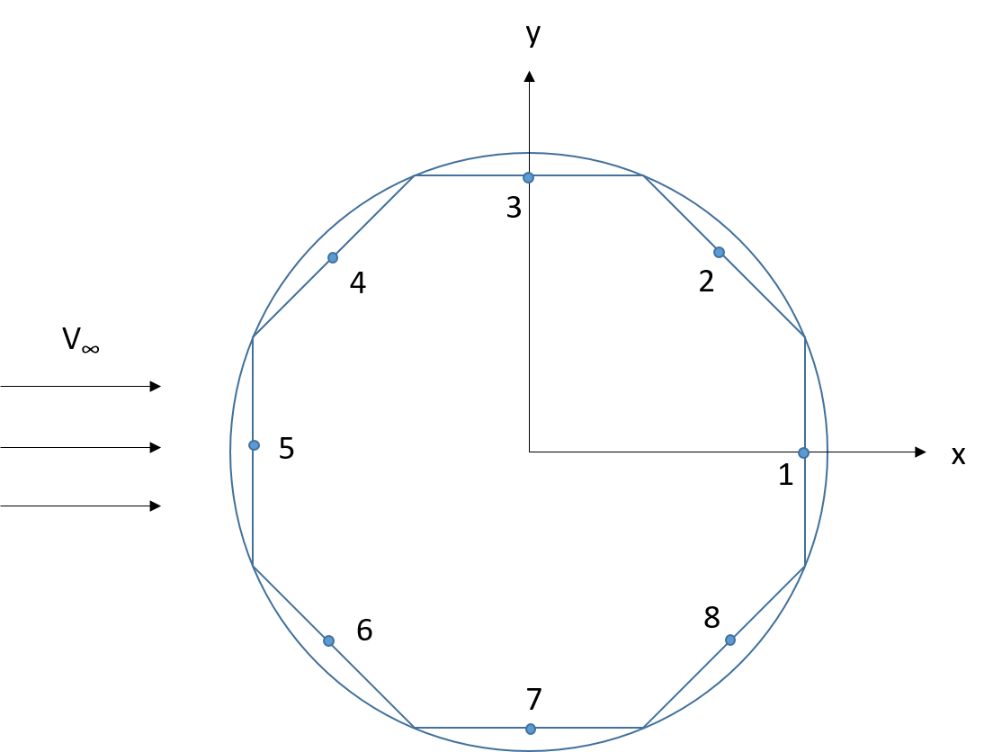
Consider the potential flow over an infinite circular cylinder. The cross section of the cylinder can be represented by a number of panels as shown in the figure. The details of the problem can be found in the book of Anderson [1].

Assume the radius $r=1$, freestream velocity $V_{\infty}=1$ and number of panels $n=8$. Lets start with initialization of the problem
import numpy as np
import matplotlib.pyplot as plt
import math as mt

r = 1               # radius of cylinder
n = 8               # number of panels
tfix = (2*mt.pi/n)  # angle between two panels
v1 = (1,0)          # freestream direction
v_inf = 1           # freestream velocity


v2    = np.zeros(2)     # surface normal vector
cp    = np.zeros(n)     # pressure coefficient
v     = np.zeros(n)     # velocity
A_mat = np.zeros((n,n)) # coefficient matrix
rhs   = np.zeros(n)     # right hand side vector
bt    = np.zeros(n)     # beta angle for each panel
phi   = np.zeros(n)     # phi angle for each panel
xe1   = np.zeros(n)     # x-coordinate of the first boundary point
xe2   = np.zeros(n)     # x-coordinate of the second boundary point
ye1   = np.zeros(n)     # y-coordinate of the first boundary point
ye2   = np.zeros(n)     # y-coordinate of the second boundary point
x1    = np.zeros(n)     # x-coordinate of the mid-point
x2    = np.zeros(n)     # y-coordinate of the mid-point
In order to apply the source panel method we need to construct the geometric properties of the panels. The coordinates of the boundary point of the panels are calculated by incrementing the $\theta$ angle in the counter clockwise direction. The $\theta$ increment is $2\pi/n$, then the boundary point coordinates are
$$X_{i+1}=\cos(i\theta+\theta/2)*r$$$$X_{i}=\cos(i\theta-\theta/2)*r$$$$Y_{i+1}=\sin(i\theta+\theta/2)*r$$$$Y_{i}=\sin(i\theta-\theta/2)*r$$The mid point coordinates are calculated as follows
$$x_{i}=\frac{X_{i+1}+X_{i}}{2}$$$$y_{i}=\frac{Y_{i+1}+Y_{i}}{2}$$The $\beta$ angle between the freestream direction ($\textbf{V}$) and the panel surface normal ($\textbf{n}$) is calculated as follows
$$\beta = \cos^{-1} \frac{\textbf{n}\cdot \textbf{V}}{|\textbf{n}||\textbf{V}|}$$for i in range(n):
theta = i*tfix
xe1[i] = mt.cos(theta+tfix/2)*r
xe2[i] = mt.cos(theta-tfix/2)*r
if theta < mt.pi/2 and theta > 3*mt.pi/2:
ye1[i] = mt.sin(theta-tfix/2)*r
ye2[i] = mt.sin(theta+tfix/2)*r
else:
ye1[i] = mt.sin(theta+tfix/2)*r
ye2[i] = mt.sin(theta-tfix/2)*r
x1[i] = (xe1[i]+xe2[i])/2
x2[i] = (ye1[i]+ye2[i])/2
nx = ye1[i] - ye2[i] # x-component of surface normal
ny = xe2[i] - xe1[i] # y-component of surface normal
v2[0] = nx
v2[1] = ny
beta = np.dot(v1,v2)/(mt.sqrt(v1[0]**2+v1[1]**2)*mt.sqrt(v2[0]**2+v2[1]**2))
beta = mt.acos(beta) # the angle between freestream and the surface normal
if ny < 0:
beta = 2*mt.pi - beta
if beta < 0:
beta = beta + 2*mt.pi
bt[i] = beta
alpha = beta - mt.pi/2
if alpha < 0:
alpha = alpha + 2*mt.pi
phi[i] = alpha
alpha = 0
beta = 0
Now we are going to apply the formulation to construct the linear system and solve for unknown vector {q}
for i in range(n):
    xi = x1[i]
    yi = x2[i]
    p1 = phi[i]
    for j in range(n):
        if i!=j:
            xj0 = xe1[j]
            xj1 = xe2[j]
            yj0 = ye1[j]
            yj1 = ye2[j]
            p2  = phi[j]

            a  = -(xi-xj0)*mt.cos(p2)-(yi-yj0)*mt.sin(p2)
            b  = (xi-xj0)**2+(yi-yj0)**2
            c  = mt.sin(p1-p2)
            d  = (yi-yj0)*mt.cos(p1)-(xi-xj0)*mt.sin(p1)
            e  = (xi-xj0)*mt.sin(p2)-(yi-yj0)*mt.cos(p2)
            sj = mt.sqrt((xj1-xj0)**2+(yj1-yj0)**2)

            iij =  (c/2)*mt.log((sj**2+2*a*sj+b)/b)+((d-a*c)/e)*(mt.atan((sj+a)/e)-mt.atan(a/e))
            A_mat[i][j] = iij/(2*mt.pi)

        A_mat[i][i] = 1/2
        rhs[i] = -v_inf*mt.cos(bt[i])

rhs = np.linalg.solve(A_mat,rhs) # solve the linear system and write the solution vector on rhs
After solving the system, we obtained the source strengths q's. Inserting the q values into the velocity equation the pressure distribution can be found as
$$C_{p}=1-\left[\frac{V_{i}}{V_{\infty}}\right]^2$$for i in range(n):
sm = 0
xi = x1[i]
yi = x2[i]
p1 = phi[i]
for j in range(n):
if i!=j:
xj0 = xe1[j]
xj1 = xe2[j]
yj0 = ye1[j]
yj1 = ye2[j]
p2 = phi[j]
a = -(xi-xj0)*mt.cos(p2)-(yi-yj0)*mt.sin(p2)
b = (xi-xj0)**2+(yi-yj0)**2
c = mt.sin(p1-p2)
d = (yi-yj0)*mt.cos(p1)-(xi-xj0)*mt.sin(p1)
e = (xi-xj0)*mt.sin(p2)-(yi-yj0)*mt.cos(p2)
sj = mt.sqrt((xj1-xj0)**2+(yj1-yj0)**2)
iij = ((d-a*c)/(2*e))*mt.log((sj**2+2*a*sj+b)/b)-c*(mt.atan((sj+a)/e)-mt.atan(a/e))
sm = sm + rhs[j]*iij/(2*mt.pi)
v[i] = v_inf*mt.sin(bt[i])+sm
cp[i] = 1 - (v[i]/v_inf)**2
To visualize the solution plot the pressure distribution on the cylinder surface. In order to obtain a more accurate solution the number of panels can be increased.
plt.xlabel(r'$\theta$')
plt.ylabel(r'$C_{p}$,v')
plt.title('Pressure coefficient distribution around the circular cylinder.')
plt.plot(bt,cp)
plt.plot(bt,v)
plt.legend(('C'r'$_{p}$', 'v'),loc='upper right')
<< 4.1 Source Panel Method || Contents || 4.2 Panel Method (Hess and Smith) >>
References:
[1] Fundamentals of Aerodynamics, J.D. Anderson, McGraw-Hill Education, 2001.