Lifting Flow Over Airfoils
Using the formulation of Hess and Smith, now we can calculate the lift around 2D bodies. Once the linear system is solved, the pressure distribution is found as in the source panel method. And the lift coefficient is calculated using the Kutta-Joukowski theorem.
$$L=\rho U \Gamma$$In here, $\Gamma=\gamma dS$ and $\gamma$ is the unique circulation value around the airfoil taht will satisfy the Kutta condition.
Assume a flow around an airfoil as shown in the figure below. Let the freestream velocity $V_{\infty}=1$ and the angle of attack $\alpha=2$. In order to apply the method we need the airfoil geometric data. For this example we are going to use NACA 4 digit series but any airfoil shape can be used. Lets start with initialization of the problem by constructing the airfoil and creating necessary arrays:
import numpy as np
import matplotlib.pyplot as plt
import math as mt
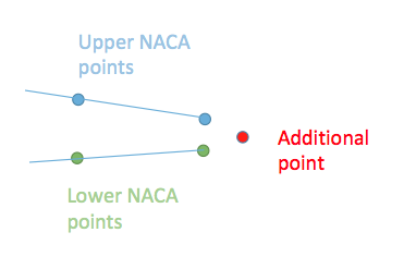
# Function for y coordinate of the additioal point at the trailing edge
def addpoint(y1,y2,y3,y4):
s1 = abs(y1-y2)
s2 = abs(y3-y4)
var = s1/s2
var = var + 1
add = (y2-y3)/var
yp = y3 + add
return yp
# NACA 4 Digit SYMMETRIC Airfoil Generation
m = 4 # maximum camber
p = 4 # maximum camber position
t = 12 # thichkness
c = 1 # chord length
strg = str(m)+str(p)+str(t) # string name for plotting
m = 0.01*m # maximum camber in % of chord
p = 0.10*p # maximum camber position in tenths of chord
t = 0.01*t # thickness in % of chord
# Coefficients for 4 digit series
a0 = 1.4845
a1 = -0.6300
a2 = -1.7580
a3 = 1.4215
a4 = -0.5075
n = 160 # number of points along the chord
npt = n*2 # number of total points along the surface
xc = np.linspace(0,c,n) # x coordinate of points along the chord
xu = np.zeros(n) # y coordinate of the upper surface
xl = np.zeros(n) # y coordinate of the upper surface
yt = np.zeros(n) # thickness distribution
yu = np.zeros(n) # y coordinate of the upper surface
yc = np.zeros(n) # y coordinate of the camber line
dyc = np.zeros(n) # gradient of the camber line
yl = np.zeros(n) # y coordinate of the lower surface
x = np.zeros(npt) # x coordinates of reordered points
y = np.zeros(npt) # y coordinates of reordered points
xi = np.zeros(npt) # x coordinate of panle mid point
yi = np.zeros(npt) # y coordinate of panel mid point
x_temp = np.zeros(npt) # temporary array
y_temp = np.zeros(npt) # temporary array
alfa = 2
alf = alfa*mt.pi/180 # angle of attack
vf = 1 # freestream velocity
ex = [1,0] # unit vector in x-direction
Re = vf*c/(1.5*10**-5)
teta = np.zeros(npt) # theta angle for each panel
A_mat = np.zeros((npt+1,npt+1)) # coefficient matrix
rhs = np.zeros(npt+1) # right hand side vector
cp = np.zeros(npt) # pressure coefficient
v = np.zeros(npt) # velocity
for i in range(n):
if (xc[i]/c < p):
yc[i] = (c*m/p**2)*(2*p*(xc[i]/c)-(xc[i]/c)**2)
dyc[i] = ((2*m)/p**2)*(p-(xc[i]/c))
else:
yc[i] = (c*m/(1-p)**2)*(1-2*p+2*p*(xc[i]/c)-(xc[i]/c)**2)
dyc[i] = ((2*m)/(1-p)**2)*(p-(xc[i]/c))
for i in range(n):
yt[i] = (t*c)*(a0*mt.sqrt(xc[i]/c)+a1*(xc[i]/c)+a2*(xc[i]/c)**2+a3*(xc[i]/c)**3+a4*(xc[i]/c)**4)
tht = mt.atan(dyc[i])
xu[i] = xc[i] - yt[i]*mt.sin(tht)
xl[i] = xc[i] + yt[i]*mt.sin(tht)
yu[i] = yc[i] + yt[i]*mt.cos(tht)
yl[i] = yc[i] - yt[i]*mt.cos(tht)
In above the 'addpoint' function calculates the $y-$coordinate of the additional point for the trailing edge, since there is a gap in the original NACA points.
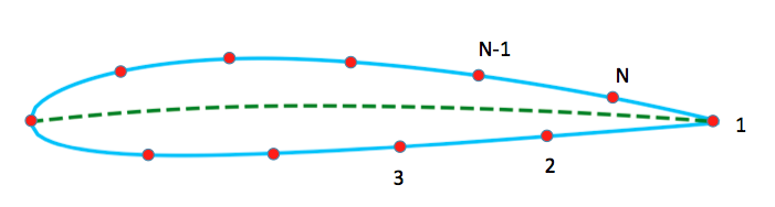
Now we need to rearange the order of the points such that the first node will be the one at the trailing edge and increase by following the lower surface as shown in the figure
for i in range(n):
    x[i]   = xu[i]
    y[i]   = yu[i]
for i in range(1,n):
    x[i+n]   = xl[n-i]
    y[i+n]   = yl[n-i]
y[n] = addpoint(y[n-2],y[n-1],y[n+1],y[n+2])
x[n] = c + c/100
x_temp[:] = x[:]
y_temp[:] = y[:]
for i in range(0,npt):
    if i<n:
        x[i] = x_temp[i+n]
        y[i] = y_temp[i+n]
    else:
        x[i] = x_temp[i-n]
        y[i] = y_temp[i-n]
del x_temp,y_temp
Notice that after creating the nodes from NACA equations there are two identical points at the leading edge and we deleted one of them. Next, we calculate the midpoints and the angles of each panel:
for i in range(npt):
    m1 = i             # first boundary point of the panel
    m2 = (i+1) % (npt) # second boundary point of the panel
    xi[i] = 0.5*(x[m1]+x[m2])
    yi[i] = 0.5*(y[m1]+y[m2])
    ty = y[m2] - y[m1]
    tx = x[m2] - x[m1]
    dot = ex[0]*tx + ex[1]*ty # dot product of two vectors
    det = ex[0]*ty - ex[1]*tx # determinant of two vectors
    teta[i] = mt.atan2(det,dot)
We are ready to construct the linear the linear system as described in the previous section:
for i in range(npt):
    p1 = teta[i]             # theta_i
    for j in range(npt):
        n1 = j               # first boundary node of  jth panel
        n2 = (j+1) % (npt)   # second boundary node of jth panel
        rij  = mt.sqrt((xi[i] - x[n1])**2+(yi[i] - y[n1])**2)  # r_ij
        rij1 = mt.sqrt((xi[i] - x[n2])**2+(yi[i] - y[n2])**2)  # r_i,j+1
        p2  = teta[j]        # theta_j
        if i==j:
            p3 = mt.pi       # beta angle
        else:
            dx1 = xi[i] - x[n1]
            dx2 = xi[i] - x[n2]
            dy1 = yi[i] - y[n1]
            dy2 = yi[i] - y[n2]
            det = dx1*dy2-dx2*dy1
            dot = dx2*dx1+dy2*dy1
            p3 = mt.atan2(det,dot)
        A_mat[i][j] = (1/(2*mt.pi))*(mt.sin(p1-p2)*np.log(rij1/rij)+mt.cos(p1-p2)*p3)
        A_mat[i][npt] = A_mat[i][npt] + (1/(2*mt.pi))*(mt.cos(p1-p2)*np.log(rij1/rij)-mt.sin(p1-p2)*p3)
        if i==0 or i==npt-1:
            A_mat[npt][j]   = A_mat[npt][j] + (1/(2*mt.pi))*(mt.sin(p1-p2)*p3-np.cos(p1-p2)*np.log(rij1/rij))
            A_mat[npt][npt] = A_mat[npt][npt] + (1/(2*mt.pi))*(mt.sin(p1-p2)*np.log(rij1/rij)+mt.cos(p1-p2)*p3)
    rhs[i] = vf*mt.sin(teta[i]-alf)
rhs[npt] = -vf*(mt.cos(teta[0]-alf)+mt.cos(teta[npt-1]-alf))
It's time to solve the system and get the $q$ and $\gamma$ values to calculate the pressure distribution and the lift coefficient:
rhs = np.linalg.solve(A_mat,rhs) # solve the linear system and write the solution vector on rhs
gamma = rhs[npt]
For the calculation of lift coefficient we will use the following formula $$L=\frac{1}{2}c_{L}\rho U^{2}c=\rho U\Gamma$$ where $\Gamma=\gamma dS$ therefore the lift coefficient is $$c_{L}=\frac{2\gamma}{cU}\sum_{i=1}^{N}S_{i}$$ And the pressure distribution is found as described in the previous chapter:
totalLength = 0
for i in range(npt):
    sum1 = 0
    sum2 = 0
    m1 = i               # first boundary node of ith panel
    m2 = (i+1) % (npt)   # second boundary node of jth panel
    totalLength = totalLength + mt.sqrt((x[m1]-x[m2])**2+(y[m1]-y[m2])**2) # total lenght of panels
    p1 = teta[i]
    for j in range(npt):
        n1 = j
        n2 = (j+1) % (npt)
        rij  = mt.sqrt((xi[i] - x[n1])**2+(yi[i] - y[n1])**2)
        rij1 = mt.sqrt((xi[i] - x[n2])**2+(yi[i] - y[n2])**2)
        p2  = teta[j]
        if i==j:
            p3 = mt.pi
        else:
            dx1 = xi[i] - x[n1]
            dx2 = xi[i] - x[n2]
            dy1 = yi[i] - y[n1]
            dy2 = yi[i] - y[n2]
            det = dx1*dy2-dx2*dy1
            dot = dx2*dx1+dy2*dy1
            p3 = mt.atan2(det,dot)
        sum1 = sum1 + (mt.sin(p1-p2)*p3-mt.cos(p1-p2)*np.log(rij1/rij))*(rhs[j]/(2*mt.pi))
        sum2 = sum2 + (mt.sin(p1-p2)*np.log(rij1/rij)+mt.cos(p1-p2)*p3)*(gamma/(2*mt.pi))
    v[i]  = vf*mt.cos(teta[i]-alf) + sum1 + sum2
    cp[i] = 1 - (v[i]/vf)**2

cl = 2*gamma*totalLength/(c*vf)
Finally, plot the pressure distribution to visualize the solution:
plt.text(0.5,0.9,'$c_{L}$=%s'%(cl))
plt.text(0.5,0.5,r'$\alpha$=%s'%(alfa))
plt.text(0.5,0.7,'$Re$=%s'%(Re))
plt.xlabel('c')
plt.ylabel(r'$C_{p}$')
plt.title('Pressure coefficient distribution around NACA %s'%strg)
plt.plot(xi,cp)
plt.gca().invert_yaxis()

<< 4.2 Panel Method of Hess And Smith || Contents || 4.2.1 Example: >>
References:
[1] An Introduction to Theoretical and Computational Aerodynemocs, Jack Moran, Dover Publications, 2010.
[2] Theoretical and Experimental Aerodynamics, Mrinal Kaushik, Springer, 2019.