DERIVATION OF CONTINUITY EQUATION
(CONSERVATION OF MASS)
The derivation of the continuity equation is based on the following physical facts:
- mass can not dissappear nor be created
- mass can only be transported by convection
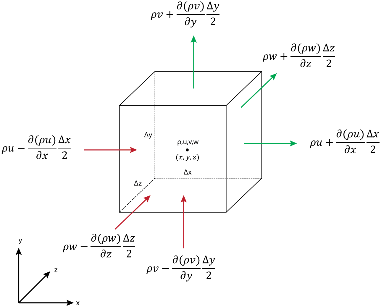
There are several approaches to derive the continuity eqaution, the following approach is the fixed fluid element model described in [1]. Consider an infinitesimally small cubic fluid element with sides $\Delta x$, $\Delta y$ and $\Delta z$. The density, $x-$, $y-$ and $z-$ velocity components at the center of the element are $p$, $u$, $v$ and $w$, respectively.
The physical meaning of the mass conversation can be written as follows
$$\left\{\begin{array}{c}
\textrm{time rate of change of }\\
\textrm{mass in fluid element}
\end{array}
\right\}=\left\{\begin{array}{c}
\textrm{mass flow into the }\\
\textrm{element from its surfaces}
\end{array}
\right\}-\left\{\begin{array}{c}
\textrm{mass flow out of the }\\
\textrm{element from its surfaces}
\end{array}
\right\}$$
Now apply this physical explanation to the given fluid element by writing mathematical descriptions for each terms above.
$$\left\{\begin{array}{c}
\textrm{time rate of change of }\\
\textrm{mass in fluid element}
\end{array}
\right\} = \frac{\partial}{\partial t}\int_{V}\rho dV \xrightarrow[\text{volume}]{\text{for fixed}}\frac{\partial}{\partial t}[\rho V]=\Delta x \Delta y \Delta z\frac{\partial \rho}{\partial t}
$$
For the calculation of mass flow (density $\times$ velocity) at the surfaces we need to use Taylor series expansion. Let the mass flux at the center of the element be $\rho u$, $\rho v$ and $\rho w$ for $x$, $y$ and $z$ direction, respectively. Then the mass flux at the center of the left and right surfaces:
$$\textrm{mass flux at the center of }x -\frac{\Delta x}{2}= \rho u - \frac{\partial (\rho u)}{\partial x}\frac{\Delta x}{2} + \frac{\partial^{2} (\rho u)}{\partial x^{2}}\frac{\Delta x^{2}}{6}-\dots$$
$$\textrm{mass flux at the center of }x+\frac{\Delta x}{2}= \rho u + \frac{\partial (\rho u)}{\partial x}\frac{\Delta x}{2} + \frac{\partial^{2} (\rho u)}{\partial x^{2}}\frac{\Delta x^{2}}{6}+\dots$$
Since we are working with an infinitesimally small element that is $\Delta x$, $\Delta y$ and $\Delta z$ are very small, we can neglect the second order and higher order terms in the Taylor series and multiplying with the area of the surface gives
$$\textrm{mass flux at }x -\frac{\Delta x}{2}= \left[\rho u - \frac{\partial (\rho u)}{\partial x}\frac{\Delta x}{2} \right]\Delta y\Delta z $$
$$\textrm{mass flux at }x+\frac{\Delta x}{2}= \left[\rho u + \frac{\partial (\rho u)}{\partial x}\frac{\Delta x}{2} \right]\Delta y\Delta z$$
Notice that the surface area for left and right surfaces are $\Delta y\Delta z$, for upper and lower surfaces are $\Delta x\Delta z$ and for back and front surfaces $\Delta x\Delta y$. Similarly the mass flux for surfaces in $y$ and $z$ directions are given as follows:
$$\left[\rho v - \frac{\partial (\rho v)}{\partial y}\frac{\Delta y}{2} \right]\Delta x\Delta z$$
$$\left[\rho v + \frac{\partial (\rho v)}{\partial y}\frac{\Delta y}{2} \right]\Delta x\Delta z$$
$$\left[\rho w - \frac{\partial (\rho w)}{\partial z}\frac{\Delta z}{2} \right]\Delta x\Delta y$$
$$\left[\rho w + \frac{\partial (\rho w)}{\partial z}\frac{\Delta z}{2} \right]\Delta x\Delta y$$
Now considering a flow in direction of positive $x$, $y$ and $z$ directions
$$\left\{\begin{array}{c}
\textrm{mass flow into }\\
\textrm{the element from}\\
\textrm{its surfaces}
\end{array}
\right\}=\left[\rho u - \frac{\partial (\rho u)}{\partial x}\frac{\Delta x}{2} \right]\Delta y\Delta z +\left[\rho v - \frac{\partial (\rho v)}{\partial y}\frac{\Delta y}{2} \right]\Delta x\Delta z + \left[\rho w - \frac{\partial (\rho w)}{\partial z}\frac{\Delta z}{2} \right]\Delta x\Delta y $$
$$\left\{\begin{array}{c}
\textrm{mass flow out of }\\
\textrm{the element from}\\
\textrm{its surfaces}
\end{array}
\right\}=\left[\rho u + \frac{\partial (\rho u)}{\partial x}\frac{\Delta x}{2} \right]\Delta y\Delta z +\left[\rho v + \frac{\partial (\rho v)}{\partial y}\frac{\Delta y}{2} \right]\Delta x\Delta z + \left[\rho w + \frac{\partial (\rho w)}{\partial z}\frac{\Delta z}{2} \right]\Delta x\Delta y $$
Combining the terms gives the following
$$\Delta x \Delta y\Delta z\frac{\partial \rho}{\partial t} = \left[\rho u - \frac{\partial (\rho u)}{\partial x}\frac{\Delta x}{2} \right]\Delta y\Delta z
+\left[\rho v - \frac{\partial (\rho v)}{\partial y}\frac{\Delta y}{2} \right]\Delta x\Delta z+\left[\rho w - \frac{\partial (\rho w)}{\partial z}\frac{\Delta z}{2} \right]\Delta x\Delta y
-\left[\rho u + \frac{\partial (\rho u)}{\partial x}\frac{\Delta x}{2} \right]\Delta y\Delta z-\left[\rho v + \frac{\partial (\rho v)}{\partial y}\frac{\Delta y}{2} \right]\Delta x\Delta z-\left[\rho w + \frac{\partial (\rho w)}{\partial z}\frac{\Delta z}{2} \right]\Delta x\Delta y $$
The terms $\pm \rho u$, $\pm \rho v$ and $\pm \rho w$ cancel each other, and $\Delta x \Delta y\Delta z$ can be dropped from the equation
$$\frac{\partial \rho}{\partial t} = \left[- \frac{\partial (\rho u)}{\partial x}\frac{1}{2} \right]
+\left[ - \frac{\partial (\rho v)}{\partial y}\frac{1}{2} \right]+\left[ - \frac{\partial (\rho w)}{\partial z}\frac{1}{2} \right] -\left[\frac{\partial (\rho u)}{\partial x}\frac{1}{2} \right]
-\left[ \frac{\partial (\rho v)}{\partial y}\frac{1}{2} \right]-\left[ \frac{\partial (\rho w)}{\partial z}\frac{1}{2} \right]$$
Rearranging the above equation gives
$$\frac{\partial \rho}{\partial t} +\frac{\partial (\rho u)}{\partial x} + \frac{\partial (\rho v)}{\partial y}+ \frac{\partial (\rho w)}{\partial z}=0$$
$$\frac{\partial \rho}{\partial t} +\nabla \cdot (\rho \textbf{U})=0 \hspace{20pt} (1)$$
This is the PDE form of the continuity equation because it was derived using an infinitesimal fluid element. This is also the conservation (or divergence) form because the element is fixed in space. Another form of the continuity equation can be written by expanding the above equation as follows
$$\frac{\partial \rho}{\partial t} + \textbf{U}\cdot \nabla \rho +\rho \nabla \cdot \textbf{U} =0$$
The first two terms correspond to the definition of material derivative for density, therefore the non-conservative form leads to
$$\frac{D \rho}{D t} +\rho \nabla \cdot \textbf{U} =0 \hspace{20pt} (2)$$
Equation (1) and (2) are same in terms of mathematics but there are significant differences when it comes to numerical discretization. If equation (2) is not properly discretized, the fluxes from the element faces do not cancel each other to the domain boundary and mass conservation is not satisfied. If the density of the fluid is constant along the flow (incompressible flow), then the gradient and time rate of change of density is zero and the continuity equation for incompressible flows reduces to
$$\nabla \cdot \textbf{U} =0 $$
<< 2.1 Substantial Derivative || Contents || 2.3 Conservation of Momentum >>
References:
[1] Computational Fluid Dynamics, J.D. Anderson, McGraw-Hill Education, 1995.
[2] Numerical Computation of Internal and External Flows: Fundamentals of Numerical Discretization, C. Hirsch, John Wiley and Sons, 1988.
[3] An Introduction to Computational Fluid Dynamics, H.K. Versteeg and W. Malalasekera, Pearson Education Limited, 2007.