Vector Differential Operator
The differential operator $\nabla$ performs on both scalar and vector fields and is called ''del'' or ''nabla''.
$$\nabla=\frac{\partial }{\partial x}\textbf{i}+\frac{\partial}{\partial y}\textbf{j}+\frac{\partial}{\partial z}\textbf{k}$$
The name of the operation depends on how it is performed on variables.
Grad:
If $f(x,y,z)$ is an differentiable function, then $\nabla f$ is the gradient of $f$
$$\nabla f=\frac{\partial f}{\partial x}\textbf{i}+\frac{\partial f}{\partial y}\textbf{j}+\frac{\partial f}{\partial z}\textbf{k}$$
Although $f$ is scalar, $\nabla f$ is a vector. Gradient tells us how a scalar quantity changes in a given direction. Here is an example python code for a contour plot of a scalar function f (first figure) and the vector field of its gradient $\nabla f$ (second figure).
import numpy as np
import matplotlib.pyplot as plot
import matplotlib.cm as cm

X = np.linspace(0,1,20)   # Create points along x-axis
Y = np.linspace(0,1,20)   # Create points along y-axis
X, Y = np.meshgrid(X, Y)  # Create 2D grid points

f   = np.sin(X)*np.cos(Y)   # Assign the function on grid points
plot.contourf(X,Y,f, 20, cmap=cm.Reds_r) # Contour plot
plot.title('Contour plot of scalar function f')
plot.show()

[gf1,gf2]=np.gradient(f) # Calculate the gradient vector of function f (grad_f)
plot.quiver(X,Y, gf1, gf2, color = ['g'],angles='xy', scale_units='xy', scale=0.75)
plot.title('Vector field of gradient of f')
plot.show()


Divergence:
Let $\textbf{F}(x,y,z)$ be a vector field, then $\textrm{div}\textbf{F}=\nabla \cdot \textbf{F}$ is the divergence of $\textbf{F}$
$$\nabla \cdot\textbf{F}=\left\{\frac{\partial }{\partial x}\textbf{i},\frac{\partial }{\partial y}\textbf{j},\frac{\partial }{\partial z}\textbf{k}\right\}\cdot
\left\{\begin{array}{c}
F_{x}\textbf{i}\\
F_{y}\textbf{j}\\
F_{z}\textbf{k}
\end{array}\right\}=\frac{\partial F_{x}}{\partial x}+\frac{\partial F_{y}}{\partial y}+\frac{\partial F_{z}}{\partial z}$$
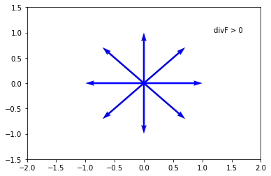
The result is a scalar and divergence of a vector fields represents how this field diverges from a point. To illustrate the physical meaning of the divergence, consider a point at the origin of the $x-y$ plane. If this point is a source, which means flow comes out from the point as seen in the figure below, then the divergence of this vector field is greater than zero at the origin and we say the flow is diverging from the source.
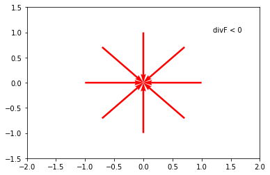
 If this point is a sink, which means flow comes in to the point as seen in the figure below, then the divergence of this vector field is less than zero at the origin and we say the flow is converging to the source.
Curl:
The curl $\nabla \times \textbf{F}$ represents the rotation of the vector field around an axis and the result is again a vector.
$$
\textrm{curl}\textbf{F}=\nabla \times \textbf{F}=\left\{\frac{\partial }{\partial x}\textbf{i},\frac{\partial }{\partial y}\textbf{j},\frac{\partial }{\partial z}\textbf{k}\right\}\times
\left\{\begin{array}{c}
F_{x}\textbf{i}\\
F_{y}\textbf{j}\\
F_{z}\textbf{k}
\end{array}\right\}=\left[\frac{\partial F_{z}}{\partial y}-\frac{\partial F_{y}}{\partial z}\right]\textbf{i}+\left[\frac{\partial F_{x}}{\partial z}-\frac{\partial F_{z}}{\partial x}\right]\textbf{j}+\left[\frac{\partial F_{y}}{\partial x}-\frac{\partial F_{x}}{\partial y}\right]\textbf{k}
$$
Laplacian:
The laplacian $\nabla^{2}$ can be performed on both scalar and vector fields. When performed on scalar, the result is a scalar and it tells how the gradient of the function changes with respect to position.
$$\nabla^{2}f=\frac{\partial^{2} f}{\partial x^{2}}+\frac{\partial^{2} f}{\partial y^{2}}+\frac{\partial^{2} f}{\partial z^{2}}$$
When the laplacian is performed to a vector field, it results in another vector field and represents the change in the flux.
$$\nabla^{2}\textbf{F}=\nabla^{2}F_{x}\textbf{i}+\nabla^{2}F_{y}\textbf{j}+\nabla^{2}F_{z}\textbf{k}$$
<< 1.1 Computational Aerodynamics || Contents || 2.1 Substantial Derivative >>