Probability Density Function

The command 'randn' produces a sample from a standard normal distribution.

z = randn

z =

    0.4847

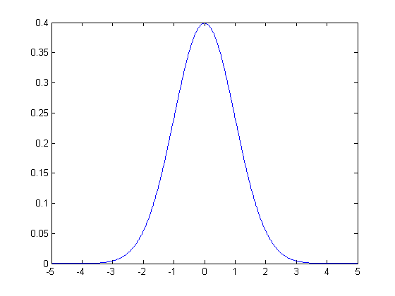
Recall that the pdf of a standard normal random variable is given by $$f_X(t) = \frac{1}{\sqrt{2\pi}}\,e^{-t^2/2}.$$ Let us sketch this function.

delta = 0.01;
t = -5:delta:5;
f = (1/sqrt(2*pi))*exp(-t.^2/2);
figure;
plot(t,f);

What does this function have to do with z above? Remember that if $\delta$ is a small positive number, we have $$ P(t-\delta/2 \leq X \leq t+\delta/2) \approx \delta \,f_X(t). $$ We can check this as follows.

N = 1000000; % draw N random variables
Z = randn(1,N);
t1 = 0.25;
% the number of the components of Z that fall in the prescribed interval,
p = sum( ( t1 - delta/2 < Z ) .* ( Z < t1 + delta/2 ) )
% the number of the components that are expected to fall in the prescribed
% interval
df = round( N * delta * (1/sqrt(2*pi))*exp( - t1^2 / 2 ) )
% p and df should be close

Suppose we repeat this for all values of t1.

ind = 0;
for t1 = t,
    ind = ind + 1;
    p(ind) = (1/delta) * (1/N)*sum( ( t1 - delta/2 < Z ) .* ( Z < t1 + delta/2 ) ) ;
end

figure;
plot(t,p,'r');
hold on;
plot(t,f);
legend('Histogram', 'pdf');

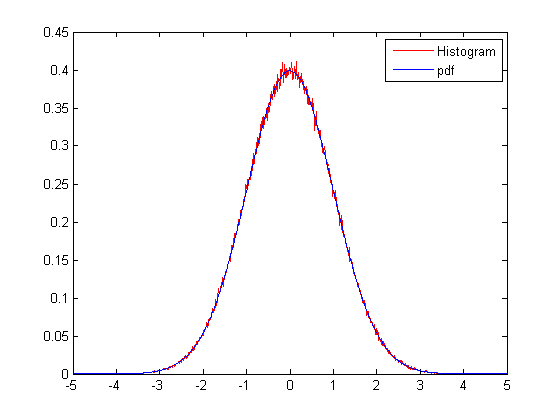
Notice how close the histogram is to the actual pdf. If we increase the size of the sample (that is, 'N'), we can obtain a histogram curve that is even closer to the pdf.

Ilker Bayram, Istanbul Teknik Universitesi, 2015